해당 자료는 전북대학교 이영미 교수님 2023고급시계열분석 자료임
library (lubridate)library (ggplot2)library (car)#library(forecast) library (lmtest)
Attaching package: ‘lubridate’


The following objects are masked from ‘package:base’:

    date, intersect, setdiff, union


Loading required package: carData

Loading required package: zoo


Attaching package: ‘zoo’


The following objects are masked from ‘package:base’:

    as.Date, as.Date.numeric
1
<- c (52 ,46 ,46 ,52 ,50 ,50 ,48 ,45 ,41 ,53 )<- length (z)
(3)
sum ((z- mean (z))^ 2 )= sum ((z- mean (z))^ 2 )/ (n-1 )
130.1
14.4555555555556
+ qt (0.975 ,(n-1 )) * sqrt ((1 + 1 / n)* s2)- qt (0.975 ,(n-1 )) * sqrt ((1 + 1 / n)* s2)
57.3206225347423
39.2793774652577
- lm함수 비교
Call:
lm(formula = z ~ 1)

Residuals:
   Min     1Q Median     3Q    Max
  -7.3   -2.3    0.7    3.2    4.7

Coefficients:
            Estimate Std. Error t value Pr(>|t|)
(Intercept)   48.300      1.202   40.17 1.83e-11 ***
---
Signif. codes:  0 ‘***’ 0.001 ‘**’ 0.01 ‘*’ 0.05 ‘.’ 0.1 ‘ ’ 1

Residual standard error: 3.802 on 9 degrees of freedom
predict (m, newdata= data.frame (t= 11 : 15 ), interval= "prediction" )
A matrix: 5 × 3 of type dbl
1
48.3
39.27938
57.32062
2
48.3
39.27938
57.32062
3
48.3
39.27938
57.32062
4
48.3
39.27938
57.32062
5
48.3
39.27938
57.32062
2
(3)
<- c (303 ,298 ,303 ,314 ,303 ,314 ,310 ,324 ,317 ,327 ,323 ,324 ,331 ,330 ,332 )<- length (z)
= 2 * (2 * n+ 1 )/ n/ (n-1 ) * sum (z) - 6 / n/ (n-1 )* sum (t* z)= 12 / n/ (n^ 2-1 )* sum (t* z) - 6 / n/ (n-1 )* sum (z)
297.780952380952
2.3857142857143
(4)
\(\hat Z_n(l) = \hat \beta_0 + \hat \beta_1(n+l)\)
+ hat_beta_1 * (15 + (1 : 5 ))
335.952380952381 338.338095238095 340.72380952381 343.109523809524 345.495238095238
- lm비교
Call:
lm(formula = z ~ t)

Residuals:
   Min     1Q Median     3Q    Max
-6.710 -2.331 -1.181  2.519  7.133

Coefficients:
            Estimate Std. Error t value Pr(>|t|)
(Intercept)  297.781      2.364 125.964  < 2e-16 ***
t              2.386      0.260   9.176 4.84e-07 ***
---
Signif. codes:  0 ‘***’ 0.001 ‘**’ 0.01 ‘*’ 0.05 ‘.’ 0.1 ‘ ’ 1

Residual standard error: 4.351 on 13 degrees of freedom
Multiple R-squared:  0.8662,    Adjusted R-squared:  0.856
F-statistic: 84.19 on 1 and 13 DF,  p-value: 4.836e-07
predict (m, newdata = data.frame (t= 15 + (1 : 5 )), interval= "prediction" )
A matrix: 5 × 3 of type dbl
1
335.9524
325.2553
346.6495
2
338.3381
327.3932
349.2830
3
340.7238
329.5084
351.9393
4
343.1095
331.6025
354.6166
5
345.4952
333.6771
357.3134
3
note: 모의시계열 표본평균과 표본분산을 안구했었네!;
<- 1 : 100 ####### (1) <- 100 + rnorm (100 ,0 ,1 )####### (2) <- 500 + rnorm (100 ,0 ,1 )####### (3) <- 100 + rnorm (100 ,0 ,10 )####### (4) <- 100 + t * rnorm (100 ,0 ,1 )
<- data.frame (Zt_1 = Zt_1,Zt_2 = Zt_2,Zt_3 = Zt_3,Zt_4 = Zt_4)round (colMeans (dt),2 )round (apply (dt,2 ,var),2 )
Zt_1 100.04 Zt_2 499.98 Zt_3 100.45 Zt_4 95.8
Zt_1 1.05 Zt_2 0.84 Zt_3 89.68 Zt_4 2449.71
ts.plot (ts (Zt_1), ts (Zt_2), ts (Zt_3), ts (Zt_4),lwd= 2 ,col= 1 : 4 )legend (c (0 ,450 ), legend = c (expression (Z[t1]), expression (Z[t2]), expression (Z[t3]),expression (Z[t4]),col= 1 : 4 , bty= 'n' , lty= 1 , lwd= 2 )
ERROR: Error in parse(text = x, srcfile = src): <text>:6:0: unexpected end of input
4: legend(c(0,450), legend = c(expression(Z[t1]), expression(Z[t2]), expression(Z[t3]),expression(Z[t4]),
5:          col= 1:4, bty='n', lty=1, lwd=2)
  ^
4
###### (1) <- 100 + rnorm (100 ,0 ,1 )####### (2) <- 100 + t + rnorm (100 ,0 ,1 )####### (3) <- 100 + 0.3 * t + sin (2 * pi* t/ 12 ) + cos (2 * pi* t/ 12 ) + rnorm (100 ,0 ,1 )
Warning message in 100 + t + rnorm(100, 0, 1):
“longer object length is not a multiple of shorter object length”
Warning message in 100 + 0.3 * t + sin(2 * pi * t/12) + cos(2 * pi * t/12) + rnorm(100, :
“longer object length is not a multiple of shorter object length”
ts.plot (ts (Zt_1), ts (Zt_2), ts (Zt_3),col= 1 : 3 , lwd= 2 )legend ("topleft" , legend = c (expression (Z[t1]), expression (Z[t2]), expression (Z[col= 1 : 3 , lty= 1 , lwd= 2 )
<- 100 + 0.3 * t + 3 * sin (2 * pi* t/ 12 ) + 20 * cos (2 * pi* t/ 12 ) + rnorm (100 ,0 ,1 )ts.plot (ts (Zt_1), ts (Zt_2), ts (Zt_3),col= 1 : 3 )legend ("topleft" , legend = c (expression (Z[t1]), expression (Z[t2]), expression (Z[col= 1 : 3 , lty= 1 )
5
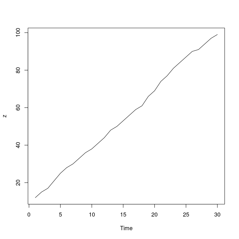
<- scan ("book.txt" )plot.ts (z)
(3)
\(Z_t = \beta_0 + \beta_1 t + \epsilon_t\)
<- 1 : length (z)<- lm (z~ t)summary (m)
Call:
lm(formula = z ~ t)

Residuals:
    Min      1Q  Median      3Q     Max
-2.5563 -1.0063 -0.2081  1.0385  2.0644

Coefficients:
            Estimate Std. Error t value Pr(>|t|)
(Intercept)  8.19080    0.46960   17.44   <2e-16 ***
t            3.07586    0.02645  116.28   <2e-16 ***
---
Signif. codes:  0 ‘***’ 0.001 ‘**’ 0.01 ‘*’ 0.05 ‘.’ 0.1 ‘ ’ 1

Residual standard error: 1.254 on 28 degrees of freedom
Multiple R-squared:  0.9979,    Adjusted R-squared:  0.9979
F-statistic: 1.352e+04 on 1 and 28 DF,  p-value: < 2.2e-16
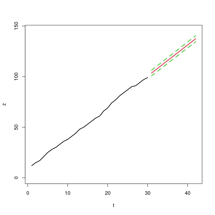
(4)
\(\hat Z_{n+l} = \hat Z_n(l) = \hat \beta_0 + \hat \beta_1(n+l)\)
<- data.frame (t= 30 + (1 : 12 ))predict (m, new_dt)
1 103.542528735632 2 106.618390804598 3 109.694252873563 4 112.770114942529 5 115.845977011494 6 118.92183908046 7 121.997701149425 8 125.073563218391 9 128.149425287356 10 131.225287356322 11 134.301149425287 12 137.377011494253
<- predict (m, new_dt, interval= "prediction" )
A matrix: 12 × 3 of type dbl
1
103.5425
100.7996
106.2855
2
106.6184
103.8584
109.3784
3
109.6943
106.9162
112.4723
4
112.7701
109.9731
115.5671
5
115.8460
113.0291
118.6629
6
118.9218
116.0842
121.7595
7
121.9977
119.1384
124.8570
8
125.0736
122.1918
127.9554
9
128.1494
125.2443
131.0546
10
131.2253
128.2960
134.1546
11
134.3011
131.3469
137.2554
12
137.3770
134.3970
140.3570
plot (t, z, type= 'n' , ylim = c (0 , 145 ), xlim= c (1 ,(30 + 12 )))lines (t, z, lwd= 2 )lines (30 + (1 : 12 ), pred[,1 ], col= 2 , lwd= 3 )lines (30 + (1 : 12 ), pred[,2 ], col= 3 , lwd= 3 , lty= 2 )lines (30 + (1 : 12 ), pred[,3 ], col= 3 , lwd= 3 , lty= 2 )
6
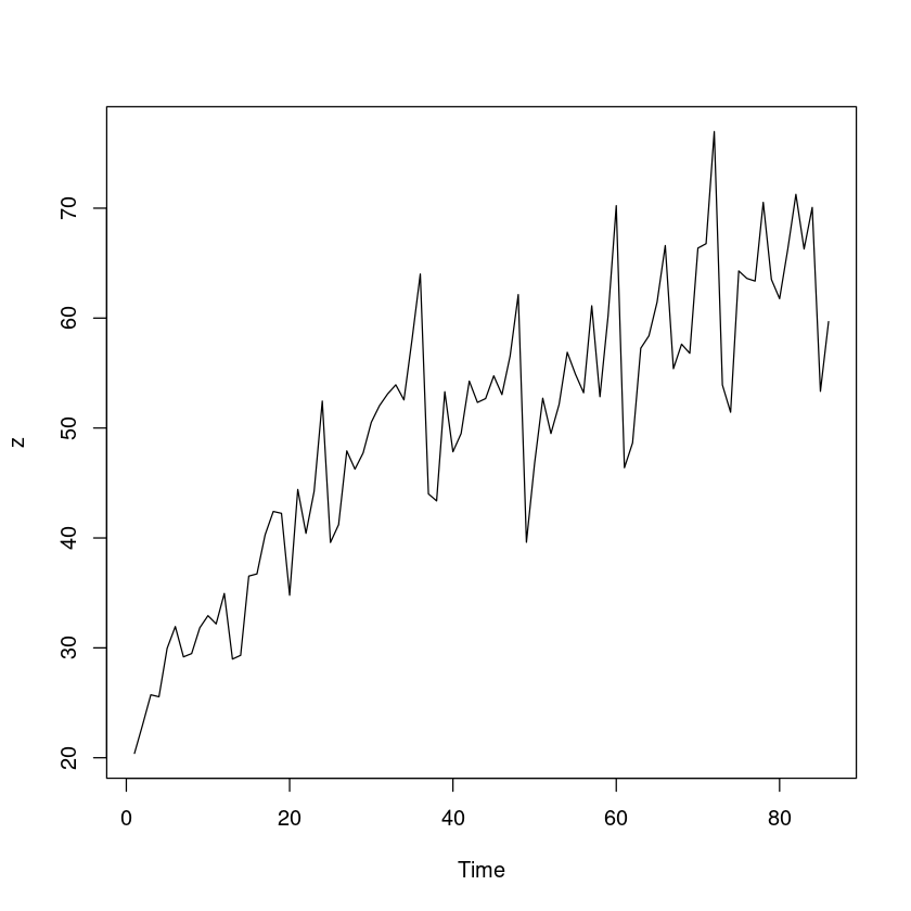
<- scan ("export.txt" )<- length (z)
86
<- ts (z, frequency= 12 )cycle (z_ts)
A Time Series: 8 × 12
1
1
2
3
4
5
6
7
8
9
10
11
12
2
1
2
3
4
5
6
7
8
9
10
11
12
3
1
2
3
4
5
6
7
8
9
10
11
12
4
1
2
3
4
5
6
7
8
9
10
11
12
5
1
2
3
4
5
6
7
8
9
10
11
12
6
1
2
3
4
5
6
7
8
9
10
11
12
7
1
2
3
4
5
6
7
8
9
10
11
12
8
1
2
추세성분, 계절성분(주기=12), 불규칙 성분으로 구성되어 있음
계절추세모형
\(Z_t = \beta_0+ \beta_1t + \sum_{i=1}^12 \delta_i \times I_{t1} + \epsilon_t\) , 단 \(\delta_1=0\)
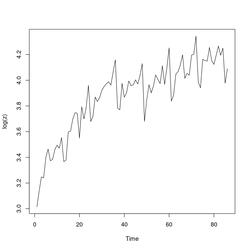
note: 나는 로그변환 한 값을 넣었음
<- ts (z, frequency= 12 )cycle (z_ts)
A Time Series: 8 × 12
1
1
2
3
4
5
6
7
8
9
10
11
12
2
1
2
3
4
5
6
7
8
9
10
11
12
3
1
2
3
4
5
6
7
8
9
10
11
12
4
1
2
3
4
5
6
7
8
9
10
11
12
5
1
2
3
4
5
6
7
8
9
10
11
12
6
1
2
3
4
5
6
7
8
9
10
11
12
7
1
2
3
4
5
6
7
8
9
10
11
12
8
1
2
<- as.factor (cycle (z_ts))<- 1 : n<- lm (z~ t+ seasonal_I)
Call:
lm(formula = z ~ t + seasonal_I)

Residuals:
     Min       1Q   Median       3Q      Max
-10.8562  -2.2938   0.1567   2.6730   9.3951

Coefficients:
             Estimate Std. Error t value Pr(>|t|)
(Intercept)  21.98000    1.73500  12.669  < 2e-16 ***
t             0.43721    0.01893  23.097  < 2e-16 ***
seasonal_I2   1.71779    2.16697   0.793 0.430512
seasonal_I3   9.21741    2.24422   4.107 0.000103 ***
seasonal_I4   7.37163    2.24366   3.286 0.001566 **
seasonal_I5   9.30299    2.24326   4.147 8.98e-05 ***
seasonal_I6  12.96578    2.24302   5.780 1.72e-07 ***
seasonal_I7   9.16286    2.24294   4.085 0.000112 ***
seasonal_I8   7.73422    2.24302   3.448 0.000941 ***
seasonal_I9  11.07272    2.24326   4.936 4.88e-06 ***
seasonal_I10 10.68409    2.24366   4.762 9.47e-06 ***
seasonal_I11 12.37545    2.24422   5.514 5.03e-07 ***
seasonal_I12 18.57967    2.24494   8.276 4.26e-12 ***
---
Signif. codes:  0 ‘***’ 0.001 ‘**’ 0.01 ‘*’ 0.05 ‘.’ 0.1 ‘ ’ 1

Residual standard error: 4.334 on 73 degrees of freedom
Multiple R-squared:  0.9011,    Adjusted R-squared:  0.8848
F-statistic:  55.4 on 12 and 73 DF,  p-value: < 2.2e-16
적합된 모형: \(\hat Z_t = 21.98 + 0.437t + 1.72 I_{t2} + 9.22 I_{t3} + \dots 18.58 I_{t12}\)
(4) 모형설명(제약조건 주의!)
1개월이 지날 때마다 월별수출액은 평균적으로 0.437억$증가
2월은 1월에 비해 월별수출액이 1.72억$ 증가
3월은 1월에 비해 월별수출액이 9.22억$ 증가
…
12월은 1월에 비해 평균 월별수출액이 18.58억$ 증가
(5)
\(\hat Z_{n+l} = \hat Z_n(l) = \hat \beta_0 + \hat \beta_1(n+l) + \sum_{i=1}^{12} \delta_i I_{t1}\)
<- data.frame ( t = n + (1 : 12 ),seasonal_I = as.factor (c (3 : 12 ,1 ,2 )))
A data.frame: 12 × 2
<int>
<fct>
87
3
88
4
89
5
90
6
91
7
92
8
93
9
94
10
95
11
96
12
97
1
98
2
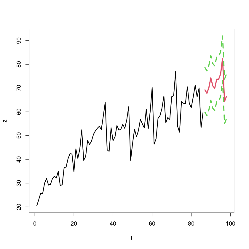
(6) 95% 예측 구간
1 69.2346153846154 2 67.8260439560439 3 70.1946153846154 4 74.2946153846154 5 70.9289010989011 6 69.9374725274725 7 73.7131868131868 8 73.7617582417582 9 75.8903296703297 10 82.5317582417582 11 64.3892994505495 12 66.5442994505494
<- predict (m2, new_dt, interval = 'prediction' )
A matrix: 12 × 3 of type dbl
1
69.23462
59.82517
78.64407
2
67.82604
58.41659
77.23549
3
70.19462
60.78517
79.60407
4
74.29462
64.88517
83.70407
5
70.92890
61.51945
80.33835
6
69.93747
60.52802
79.34692
7
73.71319
64.30374
83.12264
8
73.76176
64.35231
83.17121
9
75.89033
66.48088
85.29978
10
82.53176
73.12231
91.94121
11
64.38930
55.00439
73.77421
12
66.54430
57.15939
75.92921
69.23462 = \(\hat Z_{87} = \hat Z_{86}(1) = \hat \beta_0 + \hat \beta_1 \times 87 + \delta_3 \times I_{87 \times 3}\) (3월)
70.92890 = $ Z_{86}(5) = _0 + _1 (86+5) + 7 I {91 }$ (7월)
(7)
<- min (c (z, pred[,2 ]))<- max (c (z, pred[,3 ]))plot (t, z, type= 'n' , ylim = c (min_, max_), xlim= c (1 ,(n+ 12 )))lines (t, z, lwd= 2 )lines (n+ (1 : 12 ), pred[,1 ], col= 2 , lwd= 3 )lines (n+ (1 : 12 ), pred[,2 ], col= 3 , lwd= 3 , lty= 2 )lines (n+ (1 : 12 ), pred[,3 ], col= 3 , lwd= 3 , lty= 2 )
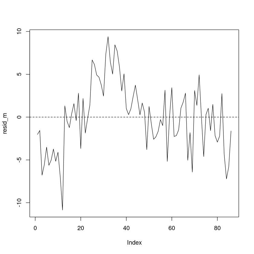
(번외) 잔차검정
<- resid (m2)plot (resid_m, pch= 16 , type= 'l' )abline (h= 0 , lty= 2 )
    One Sample t-test

data:  resid_m
t = 2.6111e-16, df = 85, p-value = 1
alternative hypothesis: true mean is not equal to 0
95 percent confidence interval:
 -0.861081  0.861081
sample estimates:
   mean of x
1.130835e-16
    studentized Breusch-Pagan test

data:  m2
BP = 18.466, df = 12, p-value = 0.1023
:: dwtest (m2, alternative= "two.sided" )
    Durbin-Watson test

data:  m2
DW = 0.79196, p-value = 5.014e-09
alternative hypothesis: true autocorrelation is not 0
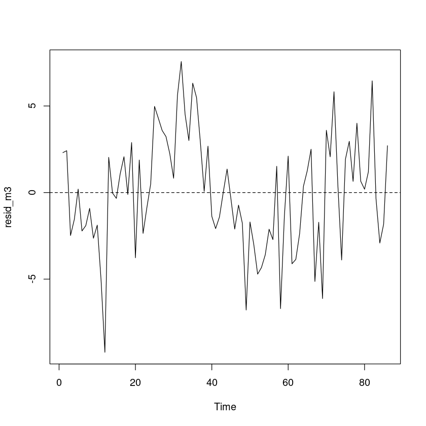
다항추세 사용
<- lm (z ~ t + I (t^ 2 ) + seasonal_I)summary (m3)
Call:
lm(formula = z ~ t + I(t^2) + seasonal_I)

Residuals:
    Min      1Q  Median      3Q     Max
-9.2252 -2.1156  0.0414  2.2895  7.5664

Coefficients:
               Estimate Std. Error t value Pr(>|t|)
(Intercept)  17.3011107  1.6527443  10.468 4.12e-16 ***
t             0.7955399  0.0637685  12.475  < 2e-16 ***
I(t^2)       -0.0041187  0.0007103  -5.799 1.65e-07 ***
seasonal_I2   1.7177908  1.8014987   0.954 0.343510
seasonal_I3   8.5584096  1.8691776   4.579 1.91e-05 ***
seasonal_I4   6.6796790  1.8690680   3.574 0.000633 ***
seasonal_I5   8.5863287  1.8690137   4.594 1.81e-05 ***
seasonal_I6  12.2326445  1.8690050   6.545 7.54e-09 ***
seasonal_I7   8.4214835  1.8690354   4.506 2.50e-05 ***
seasonal_I8   6.9928457  1.8691016   3.741 0.000365 ***
seasonal_I9  10.3395882  1.8692037   5.532 4.84e-07 ***
seasonal_I10  9.9674253  1.8693449   5.332 1.07e-06 ***
seasonal_I11 11.6835000  1.8695317   6.249 2.59e-08 ***
seasonal_I12 17.9206692  1.8697737   9.584 1.72e-14 ***
---
Signif. codes:  0 ‘***’ 0.001 ‘**’ 0.01 ‘*’ 0.05 ‘.’ 0.1 ‘ ’ 1

Residual standard error: 3.603 on 72 degrees of freedom
Multiple R-squared:  0.9326,    Adjusted R-squared:  0.9204
F-statistic: 76.58 on 13 and 72 DF,  p-value: < 2.2e-16
Call:
lm(formula = z ~ t + seasonal_I)

Residuals:
     Min       1Q   Median       3Q      Max
-10.8562  -2.2938   0.1567   2.6730   9.3951

Coefficients:
             Estimate Std. Error t value Pr(>|t|)
(Intercept)  21.98000    1.73500  12.669  < 2e-16 ***
t             0.43721    0.01893  23.097  < 2e-16 ***
seasonal_I2   1.71779    2.16697   0.793 0.430512
seasonal_I3   9.21741    2.24422   4.107 0.000103 ***
seasonal_I4   7.37163    2.24366   3.286 0.001566 **
seasonal_I5   9.30299    2.24326   4.147 8.98e-05 ***
seasonal_I6  12.96578    2.24302   5.780 1.72e-07 ***
seasonal_I7   9.16286    2.24294   4.085 0.000112 ***
seasonal_I8   7.73422    2.24302   3.448 0.000941 ***
seasonal_I9  11.07272    2.24326   4.936 4.88e-06 ***
seasonal_I10 10.68409    2.24366   4.762 9.47e-06 ***
seasonal_I11 12.37545    2.24422   5.514 5.03e-07 ***
seasonal_I12 18.57967    2.24494   8.276 4.26e-12 ***
---
Signif. codes:  0 ‘***’ 0.001 ‘**’ 0.01 ‘*’ 0.05 ‘.’ 0.1 ‘ ’ 1

Residual standard error: 4.334 on 73 degrees of freedom
Multiple R-squared:  0.9011,    Adjusted R-squared:  0.8848
F-statistic:  55.4 on 12 and 73 DF,  p-value: < 2.2e-16
2차 추세도 유의하고, 수정된 결정계수의 값이 증가 하였기 때문에 2차 추세 모형 사용 가능
plot.ts (resid_m3)abline (h= 0 , lty= 2 )
    One Sample t-test

data:  resid_m3
t = -4.2693e-16, df = 85, p-value = 1
alternative hypothesis: true mean is not equal to 0
95 percent confidence interval:
 -0.7109349  0.7109349
sample estimates:
    mean of x
-1.526557e-16
    studentized Breusch-Pagan test

data:  m3
BP = 11.389, df = 13, p-value = 0.5783
    Durbin-Watson test

data:  m3
DW = 1.1633, p-value = 4.187e-05
alternative hypothesis: true autocorrelation is greater than 0